Contents
Simple Linear Regression
Script for simple linear regression
clear
close all
clc


% get the (x_i,y_i)'s
%load IllustrationSLRdata.mat
data and model
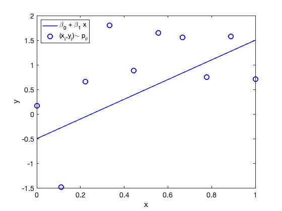
draw a sample from the SLR model with standard Gaussian noise 
%  number of observations
n = 10;

% choose a set of inputs (e.g. a grid of values in [a,b]
x = linspace(0,1,n)';

% regression coefficients $\beta_0$ and $\beta_1$
beta0 = -.5; beta1 = 2;

% Gaussian Noise parameters
mu = 0; sigma = 1;

% The true regression line
Line = beta0 + beta1 *x;

% draw a sample of noisy obervations y given x and the model parameters:

y =  Line  + normrnd(mu, sigma, n, 1);
Plot some plot options
set(0,'defaultaxesfontsize',14); %option

% plot the true regression line
plot(x, Line,'b', 'linewidth', 1.5)
xlabel('x');ylabel('y')
legend('\hat{a} \beta_0 + \beta_1 x','Location','northwest')

% together with the observed noisy pairs (x_i, y_i)
hold on
plot(x,y,'bo', 'MarkerSize',10)
legend('\beta_0 + \beta_1 x','(x_i,y_i)\sim p_\theta')
OLS estimates  and
and  for
for  and
and 
xbar = mean(x);
ybar = mean(y);

%  $\widehat\beta_1$
beta1_hat = sum((x - xbar) .* (y - ybar))/sum((x - xbar).^2);

% $\widehat\beta_0$

beta0_hat = ybar - beta1_hat*xbar;
Identical to
theta_hat = polyfit(x,y, 1);
beta1_hat = theta_hat(1);
beta0_hat = theta_hat(2);
OLS line (Predicted line)
the OLS line: 
OLS_line = beta0_hat + beta1_hat*x;
Plot the OLS line
hold on
plot(x, OLS_line,'r', 'linewidth', 2)
legend('\beta_0 + \beta_1 x','(x_i,y_i)\sim p_\theta','OLS line')

Confidenance Interval for the OLS regression line
CI_$(1-\alpha)\times 100\%$
% Risk value

alpha = 0.05;

% Value of the t-statistic
n = length(x);
tstat = tinv(1 - alpha/2, n -2); % qt(1 - alpha/2, df=n-2, lower.tail=TRUE)

% Estimate the standard deviation by its sample value
sigma_hat = std(y - (beta0_hat + beta1_hat*x)); %sqrt( sum((y - OLS_line).^2)/(n-1));

% radius of the confidence interval

r_CI = tstat*sigma_hat*sqrt(1/n + (x - xbar).^2/sum((x-xbar).^2));

IC_lwr = OLS_line - r_CI ;
IC_upr = OLS_line + r_CI;
IC = [IC_lwr, IC_upr];
Plots of the confidence region
hold on
plot(x,IC_lwr,'k--', 'linewidth', 2)
xlim([min(x), max(x)])
hold on,
plot(x,IC_upr,'k--', 'linewidth', 2)
xlim([min(x), max(x)])
legend('\beta_0 + \beta_1 x','(x_i,y_i)\sim p_\theta','OLS line',['CI\_',num2str((1-alpha)*100),'%',''])%_lwr','IC\_upr')

Another plot type: Plot with shaded region (using the boundedline function)
figure,

[hl,hp] = boundedline(x, OLS_line , r_CI , 'r-','linewidth',3, 'transparency', 0.04);
ho = outlinebounds(hl,hp);
set(ho, 'linestyle', '--', 'color', 'k');%, 'marker', '.');
hold on
h1= plot(x, Line,'b', 'linewidth', 1.5);
xlabel('x');ylabel('y')
legend(h1,'\beta_0 + \beta_1 x','Location','northwest')
hold on
h2=plot(x,y,'bo','MarkerSize',10);

legend([h1,h2,hl,hp],'\beta_0 + \beta_1 x','(x_i,y_i)\sim p_\theta','OLS Line',['CI\_',num2str((1-alpha)*100),'%',''])
box on

Prediction Interval
Value of the t-statistic
xtest = x;
nt = length(xtest);
tstat = tinv(1 - alpha/2, nt -2);

% % Estimate the standard deviation by its sample value
% sigma_hat = std(y - (beta0_hat + beta1_hat*x)); %sqrt( sum((y - OLS_line).^2)/(n-1));

% radius of the prediction interval

r_PI = tstat*sigma_hat*sqrt(1 + 1/n + (x - xbar).^2/sum((x-xbar).^2));

PI_lwr = OLS_line - r_PI ;
PI_upr = OLS_line + r_PI;
PI = [IC_lwr, IC_upr];
Plots of the prediction confidence region
Plot
figure
% plot the true regression line
plot(x, Line,'b', 'linewidth', 1.5)
xlabel('x');ylabel('y')
legend('\hat{a} \beta_0 + \beta_1 x','Location','northwest')

% together with the observed noisy pairs (x_i, y_i)
hold on
plot(x,y,'bo', 'MarkerSize',10)
legend('\beta_0 + \beta_1 x','(x_i,y_i)\sim p_\theta')

%
% Plot the OLS line
hold on
plot(x, OLS_line,'r', 'linewidth', 2)
legend('\beta_0 + \beta_1 x','(x_i,y_i)\sim p_\theta','OLS line')


% Plots of the confidence region
hold on
plot(x,IC_lwr,'k--', 'linewidth', 2)
xlim([min(x), max(x)])
hold on,
plot(x,IC_upr,'k--', 'linewidth', 2)
xlim([min(x), max(x)])
legend('\beta_0 + \beta_1 x','(x_i,y_i)\sim p_\theta','OLS line',['CI\_',num2str((1-alpha)*100),'%',''])%_lwr','IC\_upr')


% Plots of the prediction region
hold on
plot(x,PI_lwr,'r--', 'linewidth', 2)
xlim([min(x), max(x)])
hold on,
plot(x,PI_upr,'r--', 'linewidth', 2)
xlim([min(x), max(x)])
legend('\beta_0 + \beta_1 x','(x_i,y_i)\sim p_\theta','OLS line',['PI\_',num2str((1-alpha)*100),'%',''])%_lwr','PI\_upr')

Another plot type: Plot with shaded prediction region (using the boundedline function) Plot with shaded region (using the boundedline function)
figure,


[hl,hp] = boundedline(x, OLS_line , r_PI , 'r-','linewidth',3, 'transparency', 0.02);
ho = outlinebounds(hl,hp);
set(ho, 'linestyle', '--', 'color', 'r');%, 'marker', '.');
hold on
h1= plot(x, Line,'b', 'linewidth', 1.5);
xlabel('x');ylabel('y')
legend(h1,'\beta_0 + \beta_1 x','Location','northwest')
hold on
h2=plot(x,y,'bo','MarkerSize',10);

legend([h1,h2,hl,hp],'\beta_0 + \beta_1 x','(x_i,y_i)\sim p_\theta','OLS Line',['PI\_',num2str((1-alpha)*100),'%',''])
box on

hold on

[hl,hp] = boundedline(x, OLS_line , r_CI , 'r-','linewidth',3, 'transparency', 0.05);
ho = outlinebounds(hl,hp);
set(ho, 'linestyle', '--', 'color', 'k');%, 'marker', '.');
hold on
h1= plot(x, Line,'b', 'linewidth', 1.5);
xlabel('x');ylabel('y')
legend(h1,'\beta_0 + \beta_1 x','Location','northwest')
hold on
h2=plot(x,y,'bo','MarkerSize',10);

legend([h1,h2,hl,hp],'\beta_0 + \beta_1 x','(x_i,y_i)\sim p_\theta','OLS Line',['PI\_',num2str((1-alpha)*100),'%',''])
box on

Vector form
%design matrix
n=length(x);
X = [x, ones(n,1)];
beta_hat = (X'*X)^(-1)*X'*y;
Identical to:
p = 1;
theta_hat = polyfit(x,y, p);