Contents

% Risk, Bayes Risk
% Bias-Variance decomposition
% Overfitting/Underfitting
%
% (c) Faïcel Chamroukhi
%%%%%%%%%%%%%%%%%%%%%%%%%%%%
clear; close all; clc
warning off;
set(0,'defaultaxesfontsize',16); %plot option

Data generating process

% Consider the following arbitrary target function

f = @(x) 10 + 5*x.^2.*sin(2*pi*x); % the true function

plot the true function

fplot(@(x) f(x), [0, 1],'k--', 'linewidth', 1.5); xlabel('x');ylabel('y')
legend('True f(x)','Location','northeast')

Consider the following data generating process: ; for

n = 20;

% x_i's fixed or random
x = linspace(0,1, n)';

% e: independent Gaussian noise e parameters \mu_e and \sigma_e: e \sim \mathcal{N}(\mu_e, \sigma_e^2)
mu_e = 0;
sigma_e = 1;

e = normrnd(mu_e, sigma_e, n, 1);

% an example of one sample
y = f(x) + e;

An illustrating example: plot the illustrating example

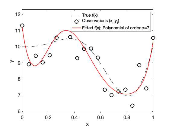
figure
% plot the true function
fplot(@(x) f(x), [0, 1],'k--', 'linewidth', 1.5); xlabel('x');ylabel('y')
legend('True f(x)','Location','northeast')

% together with the observed noisy pairs (x_i, y_i)
hold on; plot(x,y,'ko', 'MarkerSize',12)
legend('True f(x) ','Observations (x_i,y_i)')

pause

Polynomial regression

% Consider a ploynomial regression model of order p

p = 4;

% the fitted OLS function

%X = RegDesign(x, p);
beta_OLS = polyfit(x, y, p); %(X'*X)\X'*y; %inv(X'*X)*X'*y;
f_hat = @(x) polyval(beta_OLS, x);
% plot the fitted function
hold on, fplot(f_hat, [0, 1],'r-', 'linewidth', 1.5); ylim([mean(y)-2*std(y), mean(y)+3*std(y)])
legend('True f(x) ','Observations (x_i,y_i)',['Fitted f(x): Polynomial of order p=',int2str(p)])

pause

Consider ploynomial regression functions, with increasing polynomial degree , from 0 to

pmax = 14;

Examples of # polynomial fits

plot_examples = 0; if plot_examples

for p=0:pmax

compute the OLS Estimator

    beta_OLS = polyfit(x, y, p);
    % Identical to:
    %
    %   X = RegDesign(x, p);
    %   beta_OLS = (X'*X)\X'*y; %inv(X'*X)*X'*y;

compute the fitted values of the OLS function

    f_hat = @(x) polyval(beta_OLS, x);

plot the true function, together with the observed noisy pairs (x_i, y_i) and the fitted OLS function:

    figure
    % plot the true function
    fplot(@(x) f(x), [0, 1],'k--', 'linewidth', 1); xlabel('x');ylabel('y'); legend('True f(x)','Location','northeast')
    % plot the observed noisy pairs (x_i, y_i)
    hold on, plot(x,y,'ko', 'MarkerSize',12)
    legend('True f(x) ','Observations (x_i,y_i)')
    % plot the fitted OLS function
    hold on, fplot(f_hat, [0, 1],'r-', 'linewidth', 1.5); ylim([mean(y)-2*std(y), mean(y)+2*std(y)])
    legend('True f(x) ','Observations (x_i,y_i)',['Fitted f(x): Polynomial of order p=',int2str(p)])

    pause

end
% end
pause

Learn and evaluate different prediction functions

Consider N sample replicates to average the results

N = 100;

% Compute the traning and testing erros, the bias and the variance for each prediction function
Training_error  = zeros(N, pmax+1); % The training error for each sample
Testing_error  = zeros(N, pmax+1);% The prediction error for each sample

% for later computing of the biases and the variances
Hx  = zeros(n, pmax+1, N); % Matrices to store all the prediction function values
Fx  = zeros(n, pmax+1, N); % Matrices to store all the true function value

Let's consider for now a fixed design (the x's are a uniform grid in [0, 1]

x = linspace(0, 1, n)'; % for training
xtest = linspace(1/n, 1, n)'; % for testing

Draw N samples to average the results

for sample=1:N

draw a training sample

    y = f(x) + normrnd(mu_e, sigma_e, n, 1);

draw a testing sample

    ytest = f(xtest) + normrnd(mu_e, sigma_e, length(xtest), 1);

    for p=0:pmax

train the model (OLS):

        beta_OLS = polyfit(x, y, p);

fitted OLS function

        f_hat = @(x) polyval(beta_OLS, x);

Training Error (under the square loss)

        Training_error(sample,p+1) = 1/length(x) * sum((y - f_hat(x)).^2);

Testing Error (under the square loss)

        Testing_error(sample,p+1) = 1/length(xtest) * sum((ytest - f_hat(xtest)).^2);

Store the fitted h's and the trure values of the f's for later calculation of the biases and the variances

        Fx(:, p+1,  sample) = f(xtest);
        Hx(:, p+1,  sample) = f_hat(xtest);

    end

end

Plot the results

boxPlot the training error and the prediction error

figure, boxplot(Training_error), ylim([0, 7])
xlabel('Model complexity ($p$)');  ylabel('Training Error (square loss)')
figure, boxplot(Testing_error),  ylim([0, 7])
xlabel('Model complexity ($p$)');  ylabel('Prediction Error (square loss)')

% % Error and Prediction erros plotted together
% figure,subplot(121)
% boxplot(Training_error)
% ylim([0, 7])
% xlabel('Model complexity ($p$)');  ylabel('Training Error (square loss)')
% subplot(122), boxplot(Testing_error)
% xlabel('Model complexity ($p$)');  ylabel('Prediction Error (square loss)')
% ylim([0, 7])
% set(gcf,'Position',[100 500 1500 500])

pause

compute the mean errors

mean_training_error = mean(Training_error,1);
mean_testing_error = mean(Testing_error,1);

plot the mean errors

figure, plot(0:pmax, mean_training_error,'k', 'linewidth', 1.5)
hold, plot(0:pmax, mean_testing_error ,'r', 'linewidth', 1.5)
xlim([0, pmax]); ylim([0, 7])
xticks(0:pmax);
xlabel('Model complexity ($p$)')
ylabel('Error (square loss)')
legend('Mean Training Error','Mean Test Error','Location','NorthEast')

pause

Current plot held

plot the error bars

figure, errorbar(0:pmax, mean_training_error, std(Training_error,1), 'k')
hold on, errorbar(0:pmax,  mean_testing_error, std(Testing_error,1),'r')
xticks(0:pmax); xlim([0, pmax]); ylim([0, 7])
xlabel('Model complexity ($p$)')
ylabel('Error (square loss)')
legend('Training Error','Prediction Error','Location','NorthEast')

pause

Another plot type with shaded regions (using the boundedline function)

figure,
[hl,hp] = boundedline(0:pmax,  mean_testing_error, std(Testing_error,1) , 'r-','linewidth',1, 'transparency', 0.1);
hold on, plot(0:pmax,  mean_testing_error, 'k', 'linewidth', 2);
ho = outlinebounds(hl,hp);
set(ho, 'linestyle', '--', 'color', 'r');%, 'marker', '.');set(ho, 'linestyle', '-', 'color', 'r', 'marker', '.');
xticks(0:pmax); xlim([0, pmax]); ylim([0, 7])
box on
xticks(0:pmax);
xlabel('Model complexity ($p$)','interpreter','latex');
ylabel('Estimate of Risk $R = {\bf E}[(Y - h(X;\theta_p))^2]$','interpreter','latex');

%legend([h1,h2,hl,hp],'\beta_0 + \beta_1 x','(x_i,y_i)\sim p_\theta','OLS Line',['CI\_',num2str((1-alpha)*100),'%',''])
%
%%plot(0:pmax,  mean_training_error, 'k-','linewidth',2);
%%hold on,  plot(0:pmax,  mean_training_error - std(Training_error,1), 'k--', 0:pmax, mean_training_error + std(Training_error,1),'k--')
%hold on, plot(0:pmax,  mean_testing_error, 'r-','linewidth',2);
%hold on,  plot(0:pmax,  mean_testing_error - std(Testing_error,1), 'r--', 0:pmax, mean_testing_error + std(Testing_error,1),'r--')

pause

Bias-Variance Decomposition

Compute the Biases and the Variances

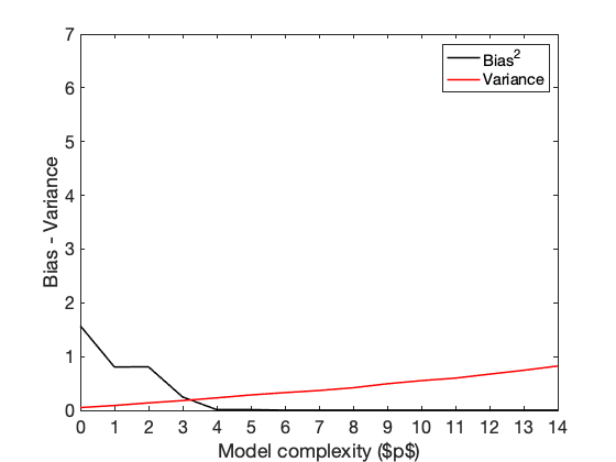
E_h =  mean(Hx, 3); % mean over the N sample replicates
B2 = zeros(n,pmax+1,N);
V = zeros(n,pmax+1,N);
for s=1:N
    B2(:,:,s) = (E_h - Fx(:,:,s)).^2;
    V(:,:,s) = (E_h - Hx(:,:,s)).^2;
end
Bias2 = mean(B2,3); % all the means^2
Variance = mean(V,3); % all the variances
%
Bias2 =  (mean(Bias2, 1)); % Bias^2
Variance = mean(Variance, 1); % Variance

% Plot the Biases and the Variances
figure, plot(0:pmax, Bias2,'k', 'linewidth', 1.5); xlim([0, pmax]);xticks(0:pmax)
hold on, plot(0:pmax, Variance,'r', 'linewidth', 1.5); xlim([0, pmax]);xticks(0:pmax)
ylim([0, 7])
xlabel('Model complexity ($p$)')
ylabel('Bias - Variance')
legend('Bias^2','Variance','Location','NorthEast')

pause

Plot all the error types together

figure, plot(0:pmax, Bias2,'k', 'linewidth', 1.5)
hold on, plot(0:pmax, Variance,'r', 'linewidth', 1.5)
hold on, plot(0:pmax, Bias2 + Variance + sigma_e^2,'b', 'linewidth', 1.5)
hold on, plot(0:pmax, mean_testing_error ,'c', 'linewidth', 1.5)
xlim([0, pmax]); xticks(0:pmax);  ylim([0, 7])
xlabel('Model complexity ($p$)')
ylabel('Errors | Bias-Variance')
legend('Bias^2','Variance', 'Bias^2 + Variance + Bayes Error','Prediction Error','Location','NorthEast')

pause

plot of bayes and prediction errors

% Bayes Error (under the square loss)

Bayes_error = sigma_e^2;

figure, plot(0:pmax, Bias2,'k', 'linewidth', 1.5)
hold on, plot(0:pmax, Variance,'r', 'linewidth', 1.5)
hold on, plot(0:pmax, Bias2 + Variance + sigma_e^2,'b', 'linewidth', 1.5)
hold on, plot(0:pmax, mean_testing_error ,'c', 'linewidth', 1.5)
hold on, plot([0 pmax], [Bayes_error Bayes_error] ,'k--', 'linewidth', 1.5)
xlim([0, pmax]); xticks(0:pmax);  ylim([0, 7])
xlabel('Model complexity ($p$)')
ylabel('Errors | Bias-Variance')
legend('Bias^2','Variance', 'Bias^2 + Variance + Bayes Error','Prediction Error', 'Bayes Error','Location','NorthEast')

pause

Plot the prediction error and the Bayes error

figure, plot([0 pmax], [Bayes_error Bayes_error] ,'k--', 'linewidth', 1.5)
hold on, plot(0:pmax, mean_testing_error ,'r', 'linewidth', 1.5)
xlim([0, pmax]); xticks(0:pmax);  ylim([0, 7])
xlabel('Model complexity ($p$)')
ylabel('Errors')
legend('Bayes Error','Prediction Error','Location','NorthEast')

Published with MATLAB® R2018a